

Method for identifying TE11 mode in TM01/TE11 mixed mode system with eight-hole coupler
-
摘要: 在高功率微波传输系统中,为了提高功率容量和效率,往往采用过模波导,因此圆波导中往往出现TM01和TE11混合模式的情况。采用角向均匀分布的8孔圆波导耦合器,对提取TE11模式的混合比和极化角度的方法进行了分析和研究。分析了圆波导中TM01和TE11模式在耦合孔处的电场分布,并采用CST对各耦合孔的输出功率进行了模拟计算,得出相互正对的耦合孔的平均功率与8个孔的平均功率之比与模式之间的相位差无关的结论。同时,发现该比值与TE11模式的混合比成线性关系,线性关系中的比例系数是极化角度线性函数。通过线性拟合获得了计算TE11模式混合比和极化方向的表达式。与仿真设定的参数相比,用该表达式计算的结果表明,在TE11模式混合比小于30%时,用其计算TE11模式的混合比和极化角度是可行的,误差不超过10%。在此基础上,给出了实际情况下TE11模式信息的具体判断方法。Abstract: In high power microwave transmission systems, over-mode waveguides are often used to improve power capacity and efficiency, thus the mixed modes of TM01 and TE11 often appear in circular waveguides. In this paper, the method of extracting the mixing ratio and polarization angle of the TE11 mode is analyzed and studied by using an 8-hole circular waveguide coupler with uniform angular distribution. The electric field distribution of the TM01 and TE11 modes in the circular waveguide at the coupling hole is analyzed, and the output power of each coupling hole is simulated by CST. By obtaining the average power of the coupling holes facing each other and the average power of the eight holes, it is concluded that the ratio is independent of the phase difference between the modes. At the same time, it is found that the ratio is linearly related to the mixing ratio of the TE11 mode, and the proportionality coefficient in the linear relationship is a linear function of the polarization angle. Expressions for calculating the TE11 mode mixing ratio and polarization direction are obtained by linear fitting. Compared with the parameters set by the simulation, the results calculated by this expression show that when the mixing ratio of TE11 mode is less than 30%, it is feasible to use it to calculate the mixing ratio and polarization angle of TE11 mode, and the error does not exceed 10%. On this basis, this paper presents a specific method for judging TE11 mode information in practical situations.
-
高功率微波(HPM)技术的不断发展[1-9]对高功率微波的功率、模式、频率等方面的测量要求越来越高。在HPM的测量技术中,HPM的在线测量是一种非常重要的测试方式和手段。HPM的在线测量不仅能够监测HPM系统的工作状态是否稳定,而且在良好标定的前提下也可以实现HPM的功率测量[10-17]。由于HPM一般在圆波导中传输,因此设置圆波导在线耦合器是常见的在线功率测量方法[18]。传统的耦合器往往只开有一个耦合孔,耦合孔内设置金属探针,将HPM功率耦合出一小部分后进行HPM功率的测量[19]。在HPM的在线测量中,除了要求对HPM功率进行测量之外,还对HPM系统内部混入的少量杂模的混合比也提出了测量的要求,而关于这方面的研究也仅限于模式的方向性测量[20],缺少确切的模式诊断方法。在实际的HPM系统中,一般使用的是圆波导TM01模式,但是由于种种原因,也往往混入了TE11模式。例如,在高功率微波系统中,为了提高功率和效率,微波系统往往采用过模波导,波导中可能激励出多种微波模式。再如,在虚阴极振荡器之类的高功率微波系统中,微波多模且模式不确定。此外在高功率微波的传输系统中,在一些不匹配连接处往往也会产生出其他干扰模式。但是这些干扰模式中,最有可能出现的是比TM01低的基模TE11模式,其他杂模如TE21和TE01等模式,仿真结果显示其含量非常小。因此,本文主要就TM01和TE11混模系统中如何提取 TE11模式信息的方法开展了研究。由于圆波导TM01模式在圆波导角向是旋转对称的,而TE11模式在角向是非对称的,因此TM01和TE11模式混合后,场分布在角向将出现非旋转对称的特点。所以,可以考虑在圆波导的角向设置多个耦合孔对TE11模式的信息进行提取。本文基于角向均匀分布的8孔耦合器进行了从TM01模式中提取TE11模式混合比和极化方向的分析和仿真研究,结果表明,采用8孔耦合器中相互正对的孔之间的平均功率,可以实现对TE11模式的混合比和极化角度进行提取,提取方法简单实用。
1. 圆波导八孔耦合器
1.1 圆波导八孔耦合器的结构
圆波导八孔耦合器采用电探针的耦合方式,于圆波导壁上,八个耦合孔沿圆波导的角向均匀分布,如图1所示。根据微波频率,耦合器被设计成只能传输TM01及以下的低次模。相比传统的单孔耦合器和三孔耦合器,八孔耦合器可以利用对向端口的平均功率对波导的传输模式进行分析和诊断。
 图 1 圆波导八孔耦合器结构示意图Figure 1. Schematic diagram of the circular waveguide eight-hole coupler structure
1.2 圆波导中TM01模式和TE11模式
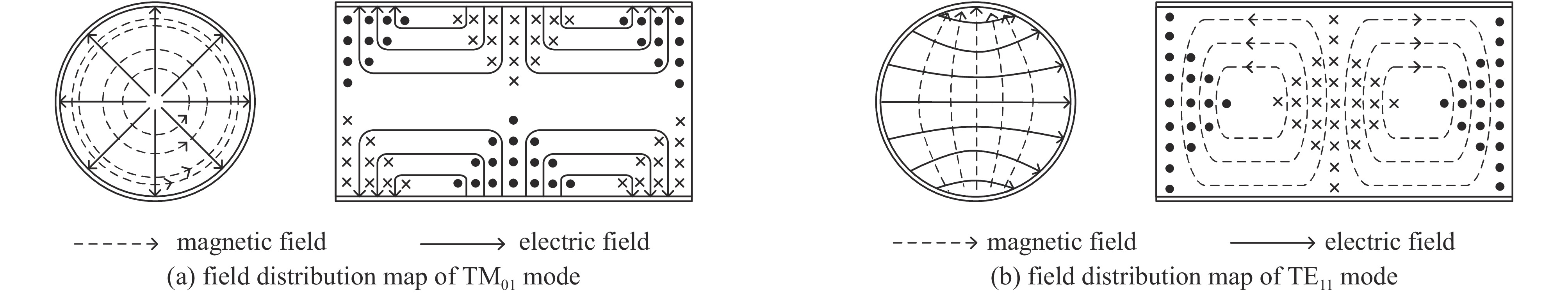
图2给出了TM01模式和TE11模式的场分布示意图,TM01模式的电场在圆波导角向均匀分布,而TE11模式的电场在圆波导中沿某种极化方向呈对称分布,因此当TM01模式混合入TE11模式时,圆波导内壁的电场强度将从均匀分布逐渐变为沿TE11极化方向对称的不均匀分布。通过对这种不均匀性变化规律进行模拟分析,可为模式混合的诊断提供指导。
2. 提取TE11模式信息的原理
2.1 混合模式在耦合孔处的电场分析
由文献[10]可知,经电探针耦合出来的功率与耦合孔处的径向电场相关。因此,在圆波导壁的耦合孔处,设ETM01、ETE11分别为TM01和TE11模式的径向电场幅度,φ1、φ2分别为TM01和TE11模式的相位,则TM01和TE11模式在耦合孔处的径向电场E01、E02分别为
{E01=ETM01sinφ1E02=ETE11sinφ2 (1) 混合模式在该处的径向电场
E=E01+E02=ETM01sinφ1+ETE11sinφ2 (2) 混合模式的径向电场也可以表示为模式幅度和相位的正弦函数,即
E=E0sin(ETM01,φ1,ETE11,φ2) (3) 其中,混合电场的幅度
E20=ETM012+ETE112+2ETM01ETE11cos(φ1−φ2) (4) 两个模式的相位差Δφ=φ1−φ2,为
tan(Δφ)=ETM01sinφ1+ETE11sinφ2ETM01cosφ1+ETE11cosφ2 (5) 考虑耦合度后,从各耦合孔检测出的功率Pi(i=1,2,…,8)为
Pi=C2TM01ETM012+C2TE11,iETE11,i2+2CTM01CTE11,iETM01ETE11,icos(Δφ) (6) 式中:C代表相应模式的耦合度。对于TM01模式,8个孔的耦合度相等,但是对于TE11模式,8个孔的耦合度是有差别的,与TE11模式的极化角度有关。
图3为耦合孔端口编号的示意图。由图2所示的TM01和TE11模式的电场分布,并结合图3的端口序号,不难看出,下列关系是成立的
 图 3 耦合孔端口序号示意图Figure 3. Schematic diagram of the serial number of the coupling hole ports
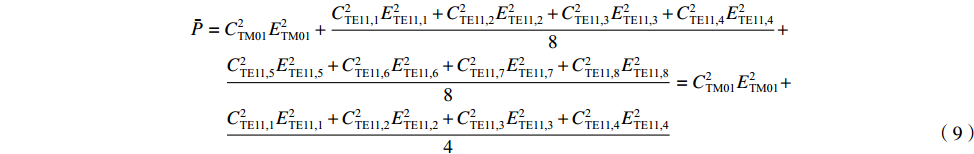
{ETE11,1=−ETE11,5ETE11,2=−ETE11,6ETE11,3=−ETE11,7ETE11,4=−ETE11,8 (7) {CTE11,1=CTE11,5CTE11,2=CTE11,6CTE11,3=CTE11,7CTE11,4=CTE11,8 (8) 将式(7)和式(8)代入式(6)后,得到8个孔的平均功率
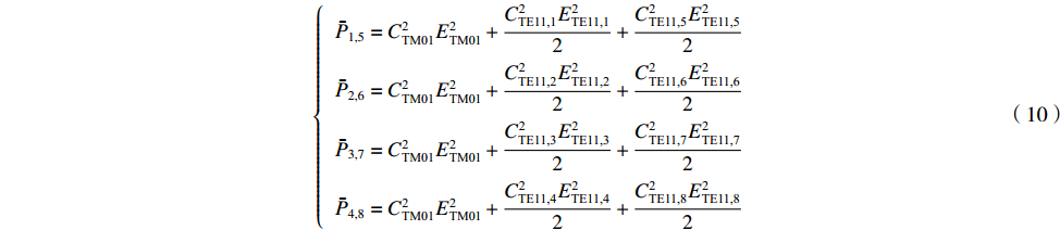
ˉP 以及相互正对孔的平均功率,即,3、7号孔的平均功率ˉP3,7 ,2、6号孔的平均功率ˉP2,6 ,4、8号孔的平均功率ˉP4,8 以及1、5号孔的平均功率ˉP1,5 分别为ˉP=C2TM01E2TM01+C2TE11,1E2TE11,1+C2TE11,2E2TE11,2+C2TE11,3E2TE11,3+C2TE11,4E2TE11,48+C2TE11,5E2TE11,5+C2TE11,6E2TE11,6+C2TE11,7E2TE11,7+C2TE11,8E2TE11,88=C2TM01E2TM01+C2TE11,1E2TE11,1+C2TE11,2E2TE11,2+C2TE11,3E2TE11,3+C2TE11,4E2TE11,44 (9) {ˉP1,5=C2TM01E2TM01+C2TE11,1E2TE11,12+C2TE11,5E2TE11,52ˉP2,6=C2TM01E2TM01+C2TE11,2E2TE11,22+C2TE11,6E2TE11,62ˉP3,7=C2TM01E2TM01+C2TE11,3E2TE11,32+C2TE11,7E2TE11,72ˉP4,8=C2TM01E2TM01+C2TE11,4E2TE11,42+C2TE11,8E2TE11,82 (10) 结果表明,上述各平均功率只是与圆波导中通过的总功率、各模式的比例以及TE11模式在各端口的耦合度有关,而与相位差无关,这对实际测量TE11模式的混合比和极化角度提供了极大的方便,这就是用8孔耦合器的原因。
2.2 提取TE11模式信息的思路
如图3所示,若TE11模式极化方向为3号端口和7号端口的连线方向,即χ=0(°)的情况,那么可以定性分析得出,随着TE11模式混合比的增加,此时3、7端口的耦合度增加,而1、5端口的耦合度减小,因此
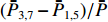
ˉP3,7 随之增加而ˉP1,5 减小。同时,由于端口的对称性,2、6号端口的耦合度与4、8端口的耦合度均相等,因此ˉP2,6=ˉP4,8 。随着TE11模式混合比的增加,ˉP3,7−ˉP1,5 逐渐增大,但始终有ˉP2,6=ˉP4,8 成立。这说明,ˉP3,7−ˉP1,5 是提取TE11模式混合比的关键。然而,在实际的微波系统中,TE11模式的极化方向通常是随机的,而极化方向又影响了各耦合孔的耦合度,因此TE11模式的极化方向对8个端口测得的功率都有影响。假定TE11模式极化方向与3端口和7端口的连线方向成χ夹角,如图3所示,此时必然
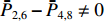
ˉP2,6−ˉP4,8≠0 ,且当TE11的极化角度增加时,ˉP2,6 与ˉP4,8 的差别越来越大。这种非对称性为判断TE11极化方向奠定了基础。另外,为了消除圆波导中总功率对各端口功率的影响,研究功率比
(ˉP2,6−ˉP4,8)/ˉP 、(ˉP3,7−ˉP1,5)/ˉP 与TE11模式混合比以及极化角度的关系,是实现对TE11模式信息提取的合理思路。3. 提取TE11模式信息的仿真研究
选取频率为9.7 GHz,采用CST仿真了8个端口的功率与TE11模式混合比和极化角度的关系。由于8个端口角向间隔为45°,因此只需要考虑χ在0°~22.5°范围内的情况即可。仿真时,圆波导中设置激励为TM01模式与TE11模式混合输入,由截止波导内的电探针采集耦合信号,即可得到各端口的功率。
3.1 相位差对端口输出功率比的影响
在圆波导中输入总功率为1 GW、TE11模式的功率为0.3 GW,即混合比ρ=30%,以及TE11模式的极化角度χ=12.5°的情况下,我们仿真了两模式之间的相位差从0~360˚变化时,8个端口的功率变化情况,并计算了相互正对端口的平均功率与8个端口平均功率的比。结果如表1所示,
ˉP1,5/ˉP 、ˉP2,6/ˉP 、ˉP3,7/ˉP 、ˉP4,8/ˉP 与相位差无关,验证了2.1的分析。表 1 功率比与相位差的关系Table 1. Relationship between power ratio and phase differenceΔφ/(°) ˉP3,7/ˉP ˉP2,6/ˉP ˉP4,8/ˉP ˉP1,5/ˉP 0 1.165 0.923 1.076 0.834 70 1.165 0.923 1.076 0.834 140 1.165 0.923 1.076 0.834 210 1.165 0.924 1.076 0.834 280 1.165 0.923 1.076 0.834 350 1.165 0.923 1.076 0.834 3.2 TE11模式的混合比和极化角度对端口输出功率比的影响
固定圆波导的输入总功率,并设两个模式的相位差为0˚,模拟了TE11模式的极化角度χ为0~22.5˚时且模式混合比ρ为0~10%时,8个端口的功率变化规律。
仿真结果显示,当圆波导中传输的为纯TM01模式时,8个端口功率基本一致。当传输的微波中混有TE11模式时,端口3与端口7功率发生明显变化,且这种变化随着TE11模式混合比增加而增大。当存在TE11模式时,端口2和端口4的功率以及端口6和端口8的功率从对称变化成非对称,且当TE11模式的极化角度增加时,这种非对称现象表现的越明显。
研究发现,
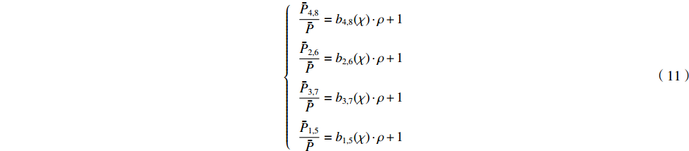
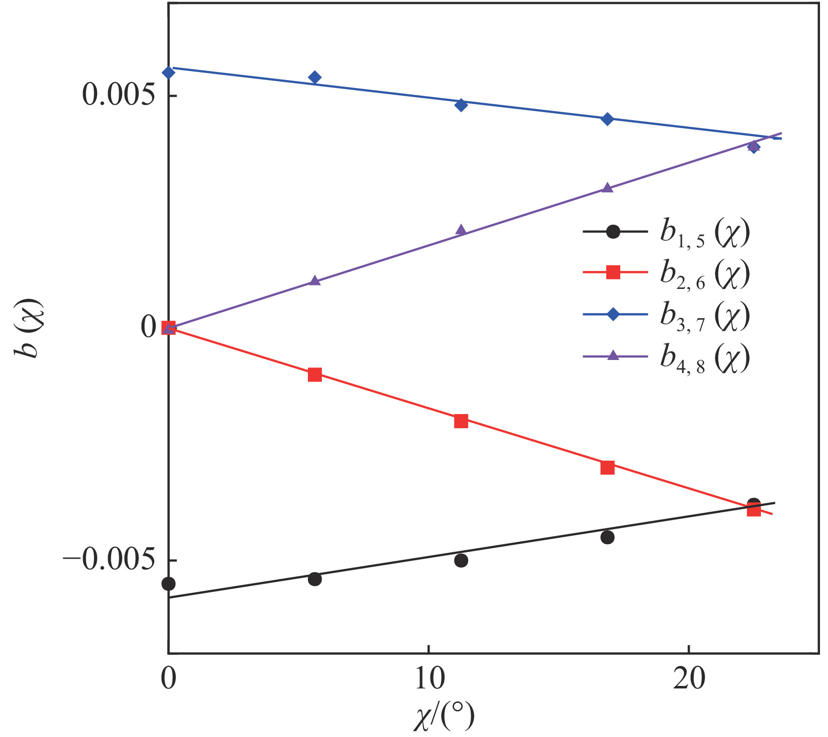
ˉP1,5/ˉP 、ˉP2,6/ˉP 、ˉP3,7/ˉP 、ˉP4,8/ˉP 都与TE11模式的极化角度χ和模式混合比ρ有关,如表2所示。由表2可以看出,在给定的混合比范围内,各功率比均可以用式(11)所示的线性关系表示,其中系数b与极化角度χ有关。表 2 功率比与极化角度和模式混合比的关系Table 2. Relationship between power ratio and polarization angle and mode mixing ratioχ/(°) ρ/% ˉP1,5/ˉP ˉP2,6/ˉP ˉP3,7/ˉP ˉP4,8/ˉP 0 0 0.999 0.999 1.000 1.000 2 0.989 1.000 1.010 1.000 4 0.978 1.000 1.021 1.000 6 0.968 0.998 1.032 1.000 8 0.956 1.000 1.043 0.999 10 0.945 1.000 1.054 0.9991 5.625 0 0.999 0.999 1.000 1.000 2 0.989 0.997 1.010 1.002 4 0.979 0.995 1.020 1.004 6 0.968 0.993 1.031 1.006 8 0.957 0.991 1.042 1.008 10 0.946 0.989 1.053 1.010 11.25 0 0.999 0.999 1.000 1.000 2 0.988 0.993 1.015 1.002 4 0.980 0.991 1.019 1.008 6 0.970 0.987 1.029 1.012 8 0.960 0.983 1.040 1.016 10 0.949 0.979 1.050 1.020 16.875 0 0.999 0.999 1.000 1.000 2 0.991 0.994 1.008 1.006 4 0.982 0.988 1.017 1.011 6 0.973 0.982 1.026 1.017 8 0.964 0.975 1.035 1.024 10 0.954 0.969 1.045 1.030 22.5 0 0.999 0.999 1.000 1.000 2 0.992 0.992 1.007 1.007 4 0.985 0.985 1.015 1.014 6 0.977 0.977 1.022 1.022 8 0.969 0.969 1.030 1.031 10 0.961 0.961 1.038 1.038 {ˉP4,8ˉP=b4,8(χ)⋅ρ+1ˉP2,6ˉP=b2,6(χ)⋅ρ+1ˉP3,7ˉP=b3,7(χ)⋅ρ+1ˉP1,5ˉP=b1,5(χ)⋅ρ+1 (11) 对表2数据进行分析后,发现b与极化角度
χ 基本上符合线性关系,如图4所示。 图 4 系数b与极化角度χ的关系Figure 4. Relationship between the proportionality coefficient b and the polarization angle χ
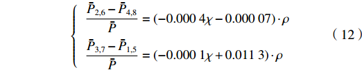
因此,根据式(11)可以得到经过数据拟合后的公式为
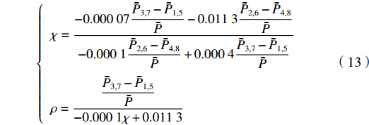
{ˉP2,6−ˉP4,8ˉP=(−0.0004χ−0.00007)⋅ρˉP3,7−ˉP1,5ˉP=(−0.0001χ+0.0113)⋅ρ (12) 由此得到计算TE11模式极化角度和混合比的表达式为
{χ=−0.00007ˉP3,7−ˉP1,5ˉP−0.0113ˉP2,6−ˉP4,8ˉP−0.0001ˉP2,6−ˉP4,8ˉP+0.0004ˉP3,7−ˉP1,5ˉPρ=ˉP3,7−ˉP1,5ˉP−0.0001χ+0.0113 (13) 式(13)表明,在实际测量中,只要我们通过8孔耦合器测量出各孔的输出功率,就可以按照式(13)计算出TE11模式的相关信息。
3.3 式(13)可行性的验证
为了验证式(13)的可行性,设置不同的相位差、TE11模式混合比和极化角度,采用CST计算出各端口的输出功率,然后按照式(13)计算出TE11模式的相关信息,并与设定值进行比较,结果如表3所示,其中ρs和χs为仿真中的设定值,ρc和χc为按照式(13)计算所得结果。
表 3 计算结果与设定值的比较Table 3. Comparison of calculation result and set valueΔφ/(°) ρs/% χs/(°) ρc/% χc/(°) Δρ/% Δχ/% values of parameters in simulation calculation results by formula-13 error 0 3 12.5 2.819 11.764 6.033 5.888 70 3 12.5 2.810 11.800 6.333 5.600 140 3 12.5 2.817 11.689 6.100 6.488 210 3 12.5 2.817 11.689 6.100 6.488 280 3 12.5 2.808 11.724 6.400 6.208 350 3 12.5 2.819 11.764 6.033 5.888 0 5 12.5 4.760 11.640 4.800 6.880 70 5 12.5 4.754 11.706 4.920 6.352 140 5 12.5 4.768 11.619 4.640 7.048 210 5 12.5 4.749 11.616 5.020 7.072 280 5 12.5 4.749 11.616 5.020 7.072 350 5 12.5 4.770 11.664 4.600 6.688 0 7 12.5 6.741 11.619 3.700 7.048 70 7 12.5 6.749 11.604 3.585 7.168 140 7 12.5 6.731 11.602 3.842 7.184 210 7 12.5 6.726 11.537 3.914 7.704 280 7 12.5 6.737 11.555 3.757 7.560 350 7 12.5 6.749 11.604 3.585 7.168 0 3 0 2.795 −0.259 6.833 70 3 0 2.802 −0.344 6.600 140 3 0 2.794 −0.344 6.866 210 3 0 2.777 −0.345 7.433 280 3 0 2.787 −0.260 7.100 350 3 0 2.806 −0.175 6.466 0 5 0 4.717 −0.225 5.660 70 5 0 4.726 −0.225 5.480 140 5 0 4.713 −0.327 5.740 210 5 0 4.711 −0.378 5.780 280 5 0 4.713 −0.327 5.740 350 5 0 4.715 −0.276 5.700 0 7 0 6.681 −0.283 4.557 70 7 0 6.669 −0.356 4.728 140 7 0 6.669 −0.356 4.728 210 7 0 6.665 −0.428 4.785 280 7 0 6.669 −0.356 4.728 350 7 0 6.685 −0.355 4.500 从表3的验算结果可以看出,用式(13)计算出的TE11模式混合比和极化角度与仿真设定的基本吻合,误差均小于10%,说明用式(13)计算TE11模式的相关信息是可行的。
4. 讨 论
4.1 式(13)的应用范围
在相位差为0的情况下,我们随机选取了对应于表4中的极化角度,在此情况下,仿真了不同混合比时,用式(13)计算出的TE11模式混合比和极化角度的相对误差。可以看出,极化角度的误差均在10%以内。当设定的混合比超过30%时,混合比的误差明显增大,并超过10%。由于实际使用中要求误差不超过10%,因此式(13)的应用范围在 0~30%之间。事实上,当 TE11 模式的混合比超过 30%之后,式(11)中的 b 与极化角度 χ 偏离线性关系,是造成误差增加的主要原因。此时,若将 b与极化角度 χ以复杂的非线性关系进行拟合的话,本文方法仍将适合于混合比超过 30%的情况。但是实际使用过程中,通过以往辐射场测量的结果显示,TE11 模式的混合比不会超过 5%,因此本文主要考虑混合比为0~10%的情况,故采用了最简单的线性拟合,以方便实际应用。
表 4 式(13)的应用范围Table 4. Application range of formula (13)ρs/% χs/(°) ρc/% χc/(°) Δρ/% Δχ/% values of parameters in simulation calculation results by formula-13 error 2 5.625 1.911 5.378 4.450 −2.343 3 12.500 2.819 11.764 6.033 5.888 4 5.625 3.851 5.143 3.725 4.005 5 12.500 4.760 11.640 4.800 6.880 6 11.250 5.795 10.407 3.416 7.493 7 12.500 6.741 11.619 3.700 7.048 8 5.625 7.895 5.085 1.312 9.600 10 16.875 9.371 16.052 6.290 4.877 30 12.500 32.653 11.510 −8.843 7.920 50 12.500 61.130 11.518 −22.26 7.856 70 12.500 97.920 11.490 −39.885 8.080 4.2 TE11模式相关信息的具体判断方法
在实际HPM情况下使用时,应避免在耦合器中通过过高的微波功率,以免造成耦合器损坏或工作不稳定。因此,选取合适的耦合孔处的倒角半径和加工光滑程度,继而提升耦合器的功率容量是非常必要的。在满足功率容量的情况下,以及在对耦合器输出功率精确测量的前提下,具体判断TE11模式的信息方法如下。
首先,用纯TM01模式的激励器,对耦合器进行耦合度的标定,也就是调整探针的位置,对耦合器的各个端口的耦合度进行调整,使其一致。
其次,在TM01和TE11混合模式下,测量各端口的输出功率。
第三,观察图1中各端口的输出功率数据是否对称,判断传输微波中是否含有TE11模式,若不对称,且最大值和最小值的连线在耦合器的某一直径线上,说明有TE11模式。
第四,依据输出功率最大值与最小值对应的端口,标出对应的3端口和7端口,并按照图3标出相应的其它端口编号。
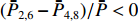
第五,利用端口2与端口4,端口6与端口8功率的非对称性,判断出极化角度落在端口3与端口7连线的某一侧。若
(ˉP2,6−ˉP4,8)/ˉP<0 ,则表示落在端口3与4之间,即图3所示的那样,反之,落在3与2之间。最后,采用用式(13),计算出TE11模式的混合比ρ和具体的极化角度χ。
5. 结 论
针对HPM系统中,圆波导中传输的TM01与TE11混合模式的实际情况,本文采用角向均匀分布的8孔耦合器,对TE11模式的混合比和极化角度等信息进行了提取方法的研究。
通过对圆波导中TM01模式和TE11模式在耦合器耦合孔处电场的分析,得出相互正对耦合孔之间的平均功率与8个孔的平均功率之比
ˉP1,5/ˉP 、ˉP2,6/ˉP 、ˉP3,7/ˉP 、ˉP4,8/ˉP 与模式之间的相位差无关,并通过CST仿真得到了验证。分析还表明,为了消除圆波导中总功率对各端口功率的影响,以功率比(ˉP2,6−ˉP4,8)/ˉP 、(ˉP3,7−ˉP1,5)/ˉP 为研究目标,更加有利于实际场合中用8孔耦合器进行TE11模式混合比和极化角度的提取,使提取方法简单实用。CST仿真结果还表明,在TE11模式的混合比小于30%的情况下,功率比
(ˉP2,6−ˉP4,8)/ˉP 、(ˉP3,7−ˉP1,5)/ˉP 正比于TE11模式的混合比ρ,比例系数b是极化角度χ的线性函数。进而给出了计算TE11模式混合比和极化方向的表达式(13)。反演结果验证了式(13)是可行的,在TE11模式混合比小于30%时,用它计算TE11模式的混合比和极化角度误差均不超过10%。
在此基础上,本文给出了实际情况下TE11模式相关信息的具体判断方法。
-
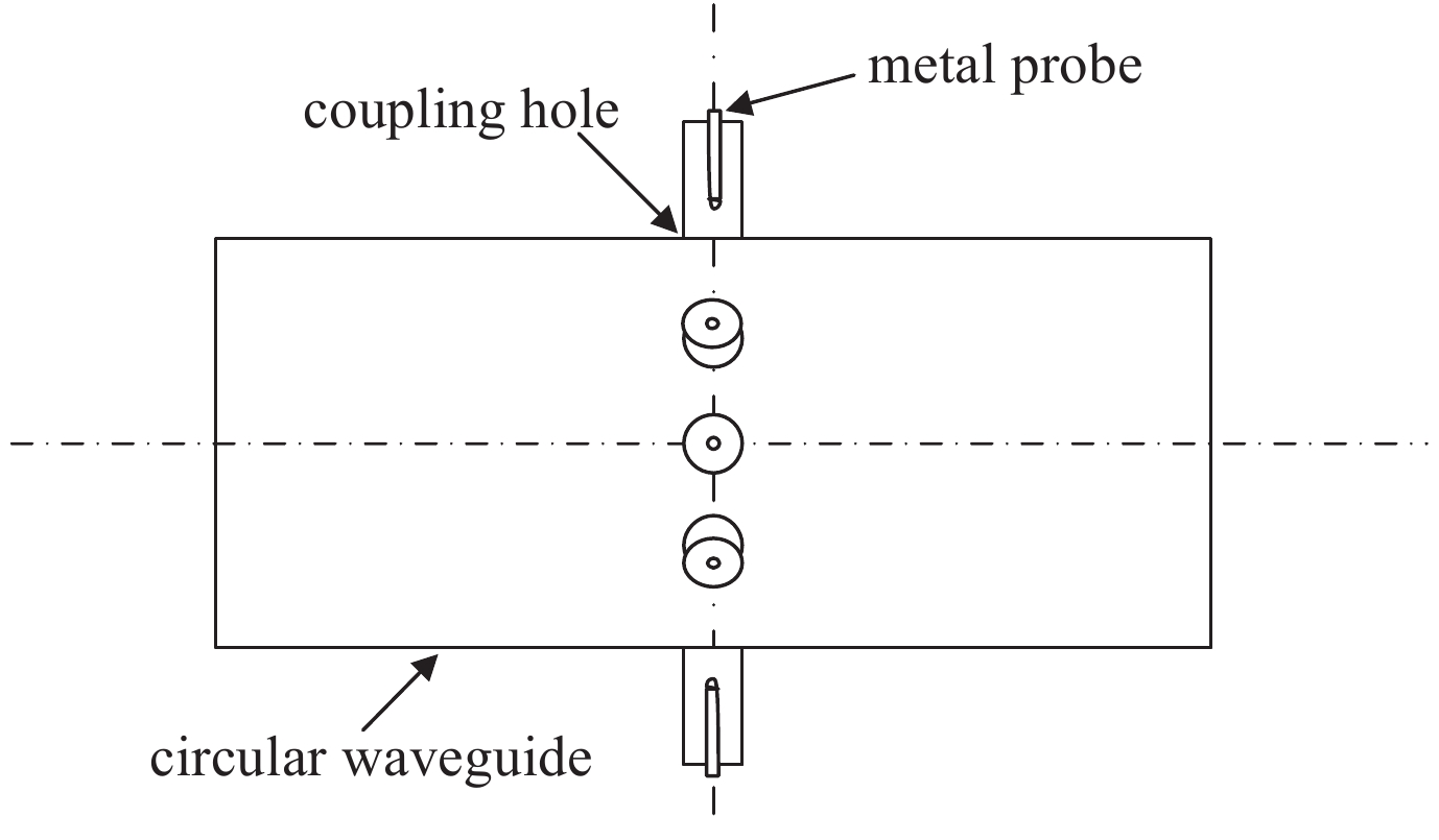
图 1 圆波导八孔耦合器结构示意图
Figure 1. Schematic diagram of the circular waveguide eight-hole coupler structure
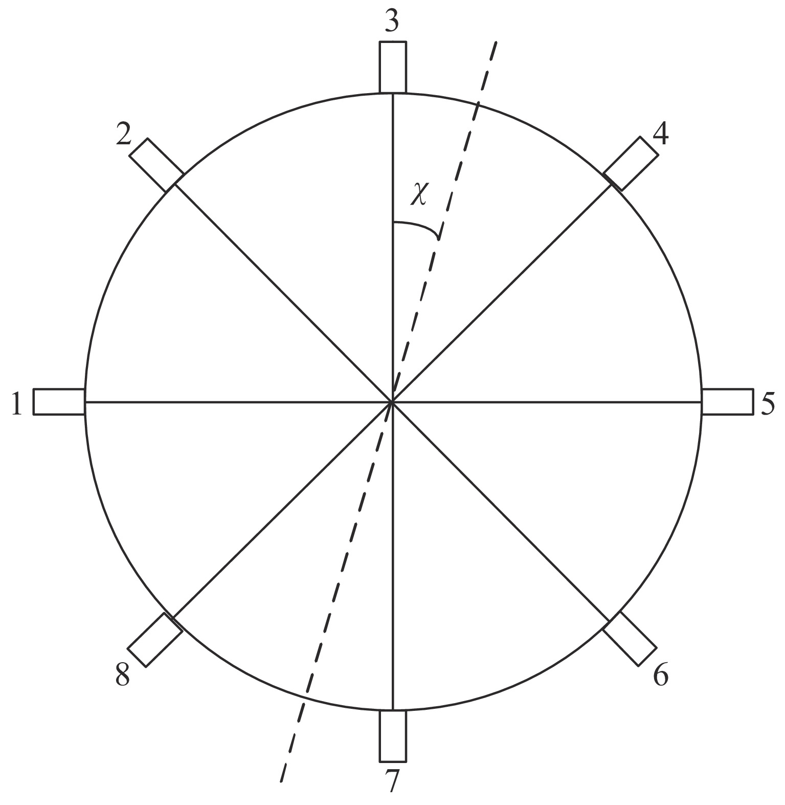
图 3 耦合孔端口序号示意图
Figure 3. Schematic diagram of the serial number of the coupling hole ports

图 4 系数b与极化角度χ的关系
Figure 4. Relationship between the proportionality coefficient b and the polarization angle χ
表 1 功率比与相位差的关系
Table 1. Relationship between power ratio and phase difference
Δφ/(°) ˉP3,7/ˉP ˉP2,6/ˉP ˉP4,8/ˉP ˉP1,5/ˉP 0 1.165 0.923 1.076 0.834 70 1.165 0.923 1.076 0.834 140 1.165 0.923 1.076 0.834 210 1.165 0.924 1.076 0.834 280 1.165 0.923 1.076 0.834 350 1.165 0.923 1.076 0.834  下载: 导出CSV
表 2 功率比与极化角度和模式混合比的关系
Table 2. Relationship between power ratio and polarization angle and mode mixing ratio
χ/(°) ρ/% ˉP1,5/ˉP ˉP2,6/ˉP ˉP3,7/ˉP ˉP4,8/ˉP 0 0 0.999 0.999 1.000 1.000 2 0.989 1.000 1.010 1.000 4 0.978 1.000 1.021 1.000 6 0.968 0.998 1.032 1.000 8 0.956 1.000 1.043 0.999 10 0.945 1.000 1.054 0.9991 5.625 0 0.999 0.999 1.000 1.000 2 0.989 0.997 1.010 1.002 4 0.979 0.995 1.020 1.004 6 0.968 0.993 1.031 1.006 8 0.957 0.991 1.042 1.008 10 0.946 0.989 1.053 1.010 11.25 0 0.999 0.999 1.000 1.000 2 0.988 0.993 1.015 1.002 4 0.980 0.991 1.019 1.008 6 0.970 0.987 1.029 1.012 8 0.960 0.983 1.040 1.016 10 0.949 0.979 1.050 1.020 16.875 0 0.999 0.999 1.000 1.000 2 0.991 0.994 1.008 1.006 4 0.982 0.988 1.017 1.011 6 0.973 0.982 1.026 1.017 8 0.964 0.975 1.035 1.024 10 0.954 0.969 1.045 1.030 22.5 0 0.999 0.999 1.000 1.000 2 0.992 0.992 1.007 1.007 4 0.985 0.985 1.015 1.014 6 0.977 0.977 1.022 1.022 8 0.969 0.969 1.030 1.031 10 0.961 0.961 1.038 1.038
下载: 导出CSV
表 3 计算结果与设定值的比较
Table 3. Comparison of calculation result and set value
Δφ/(°) ρs/% χs/(°) ρc/% χc/(°) Δρ/% Δχ/% values of parameters in simulation calculation results by formula-13 error 0 3 12.5 2.819 11.764 6.033 5.888 70 3 12.5 2.810 11.800 6.333 5.600 140 3 12.5 2.817 11.689 6.100 6.488 210 3 12.5 2.817 11.689 6.100 6.488 280 3 12.5 2.808 11.724 6.400 6.208 350 3 12.5 2.819 11.764 6.033 5.888 0 5 12.5 4.760 11.640 4.800 6.880 70 5 12.5 4.754 11.706 4.920 6.352 140 5 12.5 4.768 11.619 4.640 7.048 210 5 12.5 4.749 11.616 5.020 7.072 280 5 12.5 4.749 11.616 5.020 7.072 350 5 12.5 4.770 11.664 4.600 6.688 0 7 12.5 6.741 11.619 3.700 7.048 70 7 12.5 6.749 11.604 3.585 7.168 140 7 12.5 6.731 11.602 3.842 7.184 210 7 12.5 6.726 11.537 3.914 7.704 280 7 12.5 6.737 11.555 3.757 7.560 350 7 12.5 6.749 11.604 3.585 7.168 0 3 0 2.795 −0.259 6.833 70 3 0 2.802 −0.344 6.600 140 3 0 2.794 −0.344 6.866 210 3 0 2.777 −0.345 7.433 280 3 0 2.787 −0.260 7.100 350 3 0 2.806 −0.175 6.466 0 5 0 4.717 −0.225 5.660 70 5 0 4.726 −0.225 5.480 140 5 0 4.713 −0.327 5.740 210 5 0 4.711 −0.378 5.780 280 5 0 4.713 −0.327 5.740 350 5 0 4.715 −0.276 5.700 0 7 0 6.681 −0.283 4.557 70 7 0 6.669 −0.356 4.728 140 7 0 6.669 −0.356 4.728 210 7 0 6.665 −0.428 4.785 280 7 0 6.669 −0.356 4.728 350 7 0 6.685 −0.355 4.500
下载: 导出CSV
表 4 式(13)的应用范围
Table 4. Application range of formula (13)
ρs/% χs/(°) ρc/% χc/(°) Δρ/% Δχ/% values of parameters in simulation calculation results by formula-13 error 2 5.625 1.911 5.378 4.450 −2.343 3 12.500 2.819 11.764 6.033 5.888 4 5.625 3.851 5.143 3.725 4.005 5 12.500 4.760 11.640 4.800 6.880 6 11.250 5.795 10.407 3.416 7.493 7 12.500 6.741 11.619 3.700 7.048 8 5.625 7.895 5.085 1.312 9.600 10 16.875 9.371 16.052 6.290 4.877 30 12.500 32.653 11.510 −8.843 7.920 50 12.500 61.130 11.518 −22.26 7.856 70 12.500 97.920 11.490 −39.885 8.080
下载: 导出CSV
-
[1] Kovalev N F, Petelin M I, Raizer M D, et al. Generation of powerful electromagnetic radiation pulses by a beam of relativistic electrons[J]. Journal of Experimental and Theoretical Physics Letters, 1973, 18(4): 138-140. [2] 戴大富. 高功率微波的发展与现状[J]. 真空电子技术, 2004(5):18-24. (Dai Dafu. The present status and future developments of high power microwave[J]. Vacuum Electronics, 2004(5): 18-24 doi: 10.3969/j.issn.1002-8935.2004.05.005Dai Dafu. The present status and future developments of high power microwave[J]. Vacuum Electronics, 2004(5): 18-24 doi: 10.3969/j.issn.1002-8935.2004.05.005 [3] 曾旭, 冯进军. 高功率微波源的现状及其发展[J]. 真空电子技术, 2015(2):18-27. (Zeng Xu, Feng Jinjun. Current situation and developments of high power microwave sources[J]. Vacuum Electronics, 2015(2): 18-27Zeng Xu, Feng Jinjun. Current situation and developments of high power microwave sources[J]. Vacuum Electronics, 2015(2): 18-27 [4] He Cheng, Wu Baohua, Cai Wanyong. Discussion of UWBR and HPMW integrated design[J]. Aerospace Electronic Warfare, 2009, 25(2): 51-54. [5] 唐涛, 苏五星, 李建东, 等. 高功率雷达对抗反辐射导弹研究[J]. 空军雷达学院学报, 2012, 26(3):162-165. (Tang Tao, Su Wuxing, Li Jiandong, et al. Study on high power radar countering ARM[J]. Journal of Air Force Radar Academy, 2012, 26(3): 162-165Tang Tao, Su Wuxing, Li Jiandong, et al. Study on high power radar countering ARM[J]. Journal of Air Force Radar Academy, 2012, 26(3): 162-165 [6] 赵欲聪. Ka波段强流带状注相对论速调管放大器的高频系统研究[D]. 成都: 电子科技大学, 2014Zhao Yucong. Research on high frequency structure of KA-band intense sheet beam relativistic klystron amplifier[D]. Chengdu: University of Electronic Science and Technology of China, 2014 [7] 杨雨川. 高功率微波武器对卫星电子系统的威胁及防护技术[D]. 长沙: 国防科学技术大学, 2008Yang Yuchuan. Threaten of electronic system on satellite by HPM weapon and its protective measures[D]. Changsha: National University of Defense Technology, 2008 [8] 黄裕年. 高功率微波武器技术的发展评述[J]. 微波学报, 1999, 15(4):354-360. (Huang Yunian. Review of the progress in HPM weapon technology[J]. Journal of Microwaves, 1999, 15(4): 354-360Huang Yunian. Review of the progress in HPM weapon technology[J]. Journal of Microwaves, 1999, 15(4): 354-360 [9] Kancleris Z, Dagys M, Simniskis R, et al. Recent advances in HPM pulse measurement using resistive sensors[C]//14th IEEE International Pulsed Power Conference. 2003: 189-192. [10] 王文祥. 高功率微波功率、频率和模式的测量[J]. 真空电子技术, 2019(5):70-88. (Wang Wenxiang. Power, frequency and modes measurement of high-power microwave[J]. Vacuum Electronics, 2019(5): 70-88Wang Wenxiang. Power, frequency and modes measurement of high-power microwave[J]. Vacuum Electronics, 2019(5): 70-88 [11] 舒挺, 王勇, 李继健, 等. 高功率微波的远场测量[J]. 强激光与粒子束, 2003, 15(5):485-488. (Shu Ting, Wang Yong, Li Jijian, et al. Measurement of high power microwaves in the far-field zones[J]. High Power Laser and Particle Beams, 2003, 15(5): 485-488Shu Ting, Wang Yong, Li Jijian, et al. Measurement of high power microwaves in the far-field zones[J]. High Power Laser and Particle Beams, 2003, 15(5): 485-488 [12] 屈劲, 刘庆想, 胡进光, 等. 高功率微波辐射场功率密度测量系统[J]. 强激光与粒子束, 2004, 16(1):77-80. (Qu Jin. Liu Qingxiang, Hu Jinguang, et al. Measurement system on power density of high power microwave radiation[J]. High Power Laser and Particle Beams, 2004, 16(1): 77-80Qu Jin. Liu Qingxiang, Hu Jinguang, et al. Measurement system on power density of high power microwave radiation[J]. High Power Laser and Particle Beams, 2004, 16(1): 77-80 [13] 兰峰, 高喜, 史宗君, 等. Ka波段绕射辐射振荡器的辐射功率测量[J]. 电子科技大学学报, 2006, 35(5):777-780. (Lan Feng, Gao Xi, Shi Zongjun, et al. Measurement of radiation power for Ka-band relativistic diffraction generator[J]. Journal of University of Electronic Science and Technology of China, 2006, 35(5): 777-780 doi: 10.3969/j.issn.1001-0548.2006.05.017Lan Feng, Gao Xi, Shi Zongjun, et al. Measurement of radiation power for Ka-band relativistic diffraction generator[J]. Journal of University of Electronic Science and Technology of China, 2006, 35(5): 777-780 doi: 10.3969/j.issn.1001-0548.2006.05.017 [14] 张治强, 王宏军, 张黎军, 等. 高功率微波辐射场功率阵列测量装置研制[J]. 强激光与粒子束, 2010, 22(4):883-886. (Zhang Zhiqiang, Wang Hongjun, Zhang Lijun, et al. Development of array device for power measurement of high power microwave radiation field[J]. High Power Laser and Particle Beams, 2010, 22(4): 883-886 doi: 10.3788/HPLPB20102204.0883Zhang Zhiqiang, Wang Hongjun, Zhang Lijun, et al. Development of array device for power measurement of high power microwave radiation field[J]. High Power Laser and Particle Beams, 2010, 22(4): 883-886 doi: 10.3788/HPLPB20102204.0883 [15] 闫军凯, 刘小龙, 叶虎, 等. X波段高功率微波馈源辐射总功率阵列法测量技术[J]. 强激光与粒子束, 2011, 23(11):3149-3153. (Yan Junkai, Liu Xiaolong, Ye Hu, et al. X-band HPM feed total radiation power measurement using array method[J]. High Power Laser and Particle Beams, 2011, 23(11): 3149-3153 doi: 10.3788/HPLPB20112311.3149Yan Junkai, Liu Xiaolong, Ye Hu, et al. X-band HPM feed total radiation power measurement using array method[J]. High Power Laser and Particle Beams, 2011, 23(11): 3149-3153 doi: 10.3788/HPLPB20112311.3149 [16] 张黎军, 陈昌华, 滕雁, 等. 高功率微波辐射场远场测量方法[J]. 强激光与粒子束, 2016, 28:053002. (Zhang Lijun, Chen Changhua, Teng Yan, et al. Farfield measurement method of high power microwave in radiation field[J]. High Power Laser and Particle Beams, 2016, 28: 053002 doi: 10.11884/HPLPB201628.053002Zhang Lijun, Chen Changhua, Teng Yan, et al. Farfield measurement method of high power microwave in radiation field[J]. High Power Laser and Particle Beams, 2016, 28: 053002 doi: 10.11884/HPLPB201628.053002 [17] 刘英君, 晏峰, 景洪, 等. 高功率微波辐射场功率密度测量不确定度分析方法[J]. 电波科学学报, 2017, 32(4):398-402. (Liu Yingjun, Yan Feng, Jing Hong, et al. Measurement uncertainty on power density of high power microwave radiation[J]. Chinese Journal of Radio Science, 2017, 32(4): 398-402Liu Yingjun, Yan Feng, Jing Hong, et al. Measurement uncertainty on power density of high power microwave radiation[J]. Chinese Journal of Radio Science, 2017, 32(4): 398-402 [18] 孙钧, 胡咏梅, 张立刚, 等. 圆波导定向耦合器在高功率微波测量中的应用[J]. 强激光与粒子束, 2014, 26:063040. (Sun Jun, Hu Yongmei, Zhang Ligang, et al. Application of circular waveguide couplers in high power microwave measurement[J]. High Power Laser and Particle Beams, 2014, 26: 063040 doi: 10.11884/HPLPB201426.063040Sun Jun, Hu Yongmei, Zhang Ligang, et al. Application of circular waveguide couplers in high power microwave measurement[J]. High Power Laser and Particle Beams, 2014, 26: 063040 doi: 10.11884/HPLPB201426.063040 [19] 刘金亮, 钟辉煌, 谭启美. 同轴电探针耦合测高功率微波[J]. 微波学报, 1997, 13(1):83-87. (Liu Jinliang, Zhong Huihuang, Tan Qimei. Coaxial E-field probe coupling for high power microwave measurement[J]. Journal of Microwaves, 1997, 13(1): 83-87Liu Jinliang, Zhong Huihuang, Tan Qimei. Coaxial E-field probe coupling for high power microwave measurement[J]. Journal of Microwaves, 1997, 13(1): 83-87 [20] 陈宇, 舒挺, 郑世勇. 圆波导TE11主模辐射方向性系数的误差分析[J]. 强激光与粒子束, 2006, 18(3):431-434. (Chen Yu, Shu Ting, Zheng Shiyong. Error analysis of radiation directivity of TE11 main mode of circular waveguide[J]. High power Laser and Particle Beams, 2006, 18(3): 431-434Chen Yu, Shu Ting, Zheng Shiyong. Error analysis of radiation directivity of TE11 main mode of circular waveguide[J]. High power Laser and Particle Beams, 2006, 18(3): 431-434 期刊类型引用(3)
1. 陈家辉,周振宇,翁明,曹猛. 圆波导TM_(01)模式转换器中TE_(11)和TE_(21)模式对圆波导耦合器耦合度的影响. 真空科学与技术学报. 2024(06): 492-502 .  百度学术
百度学术2. 雷乐,周振宇,翁明,林舒,曹猛. S波段矩形波导TE_(10)-圆波导TM_(01)模式转换器的研究. 真空科学与技术学报. 2023(06): 537-546 . 百度学术3. 周振宇,陈家辉,翁明,林舒,曹猛. 同轴横电磁波转圆波导横磁波01模式的转换器研究. 西安交通大学学报. 2023(11): 171-180+205 . 百度学术其他类型引用(0)
-


 下载:
下载:


 点击查看大图
计量
- 文章访问数: 885
- HTML全文浏览量: 283
- PDF下载量: 69
- 被引次数: 3
