

Evolution of explosion plume on the rear surface of silica elements in nanosecond laser damaging
-
摘要: 紫外光学元件损伤动力学的研究是关联物质微观结构演化与光学元件宏观性质变化的重要纽带。在光学元件后表面损伤坑形成的过程中,激光能量沉积导致材料爆炸形成高温高压物质突破表面,并伴随形成爆炸流场和喷溅射流。爆炸流场与初始起爆强度具有强关联性,对爆炸流场及喷溅行为进行研究,可以帮助分析损伤初期的材料状态变化和响应机制,是损伤动力学研究的必需环节。基于多种时间分辨成像技术,捕获了损伤发展前期的材料电离和气化响应演化行为,分析了材料损伤起爆后气化电离等过程的弛豫时间,并确定各个行为转化的关键时间节点,描述了损伤区域能量快速释放的物理过程。Abstract: The study of UV laser induced damage dynamics is the key to exploring correlating evolution of optical elements’ microstructure and macroscopic properties. In optical elements damage process on the rear surface, the laser energy deposition causes the material to explode with high pressure and high temperature to break through the rear surface, and it is accompanied with explosion plume and jet particles. The explosion plume is greatly affected by the initial laser energy deposition. The study of the explosion plume can help a lot in analyzing the material state change and response mechanism at the initial stage of damage. In this paper, explosion plume on the rear surface is investigated using a two-color interferometric time-resolved side-viewed imaging system. Assisted with the observation of the collected ejection, the material species, distributions and thermodynamic behaviors of ejections are presented. Based on findings, the key transition nodes of the response behaviors during laser induced damage formation are captured and the temporal evolvement of plume is described.
-
Key words:
- optical elements damage /
- fused silica /
- explosion plume /
- particle jet /
- damage dynamics
-
High-resolution flow field data play an important role in fluid mechanics, fluid dynamics research, engineering design and technological innovations. Accurate acquisition and analysis of high-resolution flow field data is of great significance for understanding flow phenomena. There are two main ways to obtain high-resolution flow field data, one is experimental measurements, such as Particle Image Velocimetry (PIV)[1], the other is Computational Fluid Dynamics (CFD)[2], such as Direct Numerical Simulation (DNS)[3-5]. However, obtaining high-resolution flow field data through experiments or CFD is either costly or time-consuming, thus new methods need to be developed.
Artificial intelligence technology has been booming unprecedentedly nowadays[6]. As the main method of artificial intelligence, Convolutional Neural Networks (CNN)[7] has been widely used in various fields and promoted many innovations and progress. CNN is a deep learning model inspired by the biological vision system. The development of CNN has experienced many milestones. The earliest CNN model can be traced back to the 1990s, such as LeNet[8] proposed by LeCun for handwritten digit recognition. In the 2012 ImageNet Large-Scale Visual Recognition Challenge, the emergence of the AlexNet[9] model has greatly promoted the development of CNN, which uses a deeper networks structure and a large amount of image data for training, and achieved breakthrough results. Since then, various improved CNN models have emerged, such as VGGNet[10], GoogLeNet[11], ResNet[12], etc., which have achieved excellent performance in different computer vision tasks.
The vigorous development of CNN has been spread to various fields, including fluid mechanics. Especially in recent years, fluid mechanics has been closely combined with CNN. In 2018, Jin et al designed a fused CNN model[13]. Through this model, the velocity field around the cylinder can be predicted only according to the pressure fluctuation on the cylinder. This model has good performance under different Reynolds numbers. In 2019, Sekar et al first used CNN to extract the geometric features of the airfoil[14], and to predict the flow field around the airfoil through the fully connected layer with the help of other state information. In the direction of high-resolution reconstruction of the flow field, Fukaimi et al proposed a hybrid Down sampled Skip-Connection Multi-Scale model to reconstruct the flow field[15] in 2019. In this model, only dozens of training samples are used to produce a good performance. At the same year, Deng et al constructed two models based on generative adversarial networks to enhance the spatial resolution of the complex wake behind two side-by-side cylinders[16]. In 2020, Liu et al developed the multi-time-path CNN model for high-resolution reconstruction of turbulence[17]. In 2021, Zhou et al used the geometric parameters of the coarse velocity field and the pore structure as the input of the CNN model to achieve super-resolution reconstruction of the pore flow field in porous media[18]. In 2022, Jagodinski et al designed a three-dimensional CNN model to identify significant structures related to ejection events in wall-bounded turbulent flows[19].
The ablative Rayleigh–Taylor instability (ARTI)[20] flow field data is mainly obtained by numerical simulations and experiments. At present, high-precision simulation requires fine meshing, however, it is costly and time-consuming. Low-precision simulation takes a short time, but it cannot describe the physical characteristics of the flow field in detail. Therefore, we need to develop a new method that can obtain high-precision ablation Rayleigh-Taylor instability flow field data at a relatively small computational cost. In this study, two different CNN models are given out to perform the high-resolution reconstruction. These two models can quickly transform low-resolution data into high-resolution data, which allows us to obtain high-resolution ARTI flow field data rapidly.
1. Methods
1.1 ARTI and DNS
The Rayleigh–Taylor instability (RTI) occurs at the perturbation interface of two fluids with different densities, where the light fluid accelerates or supports the heavy fluid[21]. In inertial confinement fusion (ICF), RTI can break the symmetry of implosions by dismantling the integrity of the spherical ablator-fuel shell. Therefore, it is crucial to predict the growth of RTI to improve the success probability of ICF. The inclusion of thermal conduction influences leads to a different hydrodynamic instability, which is then identified as ARTI, occurring between the internal and external layers during the implosion phase of ICF[22].
The control equations of the ARTI over a constantly accelerating 2D reference frame are as follows
∂tρ=−∂x(ρu)−∂y(ρv), (1) ∂t(ρu)=−∂x(ρu2+p)−∂y(ρuv)+ρg, (2) ∂t(ρv)=−∂x(ρuv)−∂y(ρv2+p), (3) ∂t(ρe)=−∂x[(ρe+p)u]−∂y[(ρe+p)v]+∂x(κ∂xT)+∂y(κ∂yT)+ρug, (4) where
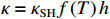
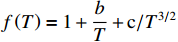
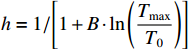
ρ , u, v and T represent density, x-axis velocity component, y-axis velocity component and temperature, respectively. g is acceleration,p=ΓρT is the pressure, ande=CvρT+ρv22 is the total energy, whereCv=Γ/(γh−1) is the constant-volume specific heat. For CH material,γh=5/3 andΓ=57.51cm2/(μs2⋅MK) .κ=κSHf(T)h is the coefficient of thermal conductivity, whereκSH∝T5/2 is the classical electron thermal conductivity coefficient.f(T)=1+bT+c/T3/2 is the preheating function, andh=1/[1+B⋅ln(TmaxT0)] because there is a large temperature gradient near the critical surface,T0 andTmax are the initial electron temperature and the maximum electron temperature, respectively, in the corona region, and B is an adjustable parameter, usuallyB=1 . For the strong preheat case discussed in this paper, we set h=1, b=8.6, c=1.6.The data used in this work are derived from the DNS of ARTI in Ref.[4], and the Euler code which has been usually applicated in high energy density physics is used in our study. Before the formal training of the CNN model, we process the original DNS data through region selection, dislocation stitching, pooling and other processes to obtain the sample data. In this paper, both maximum pooling and average pooling are used to implement down-sampling.
1.2 Two CNN models
In this paper, the application of ordinary CNN model and multi-time-path CNN model are discussed, and the results are also compared with those of the BiCubic interpolation method[23].
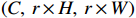
The ordinary CNN model consists of three convolution layers and an up-sampling layer, as shown in Fig.1. The input of the model is the low-resolution flow field data and the output is the high-resolution flow field data at the same time. The role of the convolution layer is to extract the characteristics of the flow field data. The size of the convolution kernel is
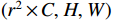
3×3 . The function of the up-sampling layer is to integrate and enlarge the feature maps obtained by convolution operation, so as to achieve high-resolution reconstruction. The PixelShuffle up-sampling method[24] is adopted to transform the feature map with the input size of(r2×C,H,W) into the flow field map with the input size of(C,r×H,r×W) by pixel recombination of the low-resolution feature map,where r is the reconstruction magnification, C is the number of channels, H is the height of the feature map, W is the width of the feature map. Figure 1. Schematic diagram of ordinary CNN structure
The second model is a multi-time-path CNN. The schematic diagram of the model is shown in Fig.2.
 Figure 2. Schematic diagram of the structure of a multi-time-path CNN
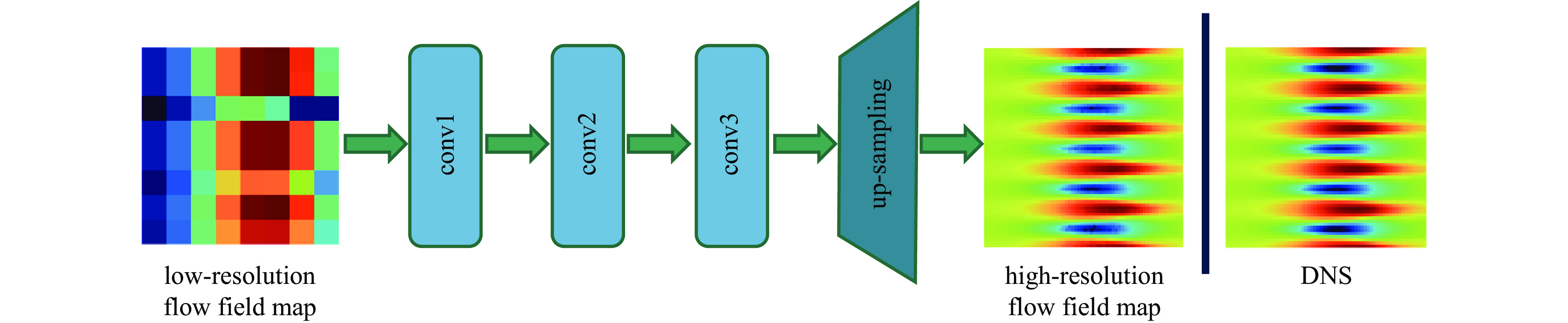
The input of the multi-time-path CNN is the low-resolution flow field data of the five moments at
t−2Δt ,t−Δt , t,t+Δt ,t+2Δt respectively and the output is the high-resolution flow field data of the moment t. The model includes four paths, three of which are time paths and the other is the weight path. The time paths include the backward time path, central time path and forward time path. The input of each time path is the low-resolution flow field data at three consecutive moments. The input of the backward time path is the flow field data at three moments oft−2Δt ,t−Δt , t. The input of the central time path is the flow field data at three moments oft−Δt , t,t+Δt . The input of the forward time path is the flow field data at three moments of t,t+Δt ,t+2Δt . Therefore, a set of input data of the model contains low-resolution flow field data at five moments. The structures of all the time paths are the same, including feature extraction module and reconstruction module. The feature extraction module consists of two basic blocks, each of which is an enhanced multi-scale residual block[25], and a jump connection method is used on each time path to avoid the loss of features caused by convolution operations. In the weight path, the input is the feature maps extracted by the feature extraction module of the three time paths, and the output is three weight maps. The summation of the products of the obtained weight map and the reconstructed flow field map obtained by the three time paths will finally give the high-resolution flow field map at the moment t. In other words, the final high-resolution flow field data is actually the weighted average of the high-resolution flow field data obtained by the three time paths.Compared with the ordinary CNN, multi-time-path CNN has more input data and more complex networks structure, thus the expected results should also be better than those of the ordinary CNN. It is worth mentioning that the multi-time-path CNN takes the time series as the model input, combines the timing of the flow field changing with time, and has the superiority that the ordinary CNN cannot achieve.
1.3 Model training
After a series of data processing, we randomly divided
2000 samples into 80% training set (1600 samples) and 20% test set (400 samples). Taking a magnification of 4 as an example, the input size of our ordinary CNN model is [C, 16, 16], and the input size of the multi-time-path CNN is [3, C * 3, 16, 16]. Because the multi-time-path CNN has three paths, there is an additional dimension on the input scale. Each path of the multi-time-path CNN contains data of three moments, thus, the number of channels is C * 3. The last two dimensions represent the height and width of the feature map. We set the batch size to be 32 and Epoch to be 2000.Before putting into training, the input data should be normalized, which will make the model converge faster. We select activation function as the ReLU function, which is often used in neural networks. Because our super-resolution reconstruction task is actually a regression task, we cannot use the activation function in the last convolution layer. For weight initialization, we also use the corresponding initialization method of ReLU function.
The loss function in the above two models is written as
L=∑Ni=1(Hi−Pi)2N, (5) where L is also called as Mean Square Error (MSE), N is the number of data point, H, P are the real value and the predicted value of the point, respectively.
All the models in this paper are in Python, which mainly depends on PyTorch to realize the construction of CNN model. As for gradient update, Adam[26] (Adaptive Moment Estimation) optimization algorithm is used to adaptively adjust the parameters in the neural networks, which can converge to the optimal solution quickly. In the parameter setting of Adam, we choose the learning rate 0.0001. The training process of the model involves iterating through 2000 epochs. The ordinary CNN takes 4 h and 2 min, and the multi-time-path CNN takes 4 h and 23 min. The structure of the multi-time-path CNN is more complex and has more parameters than the ordinary CNN, thus requiring a slightly longer computation time. After the model training is completed, the high-resolution reconstruction task can be achieved in a few seconds.
2. Results and analysis
The DNS data used here are ARTI flow field data with a disturbance wavelength
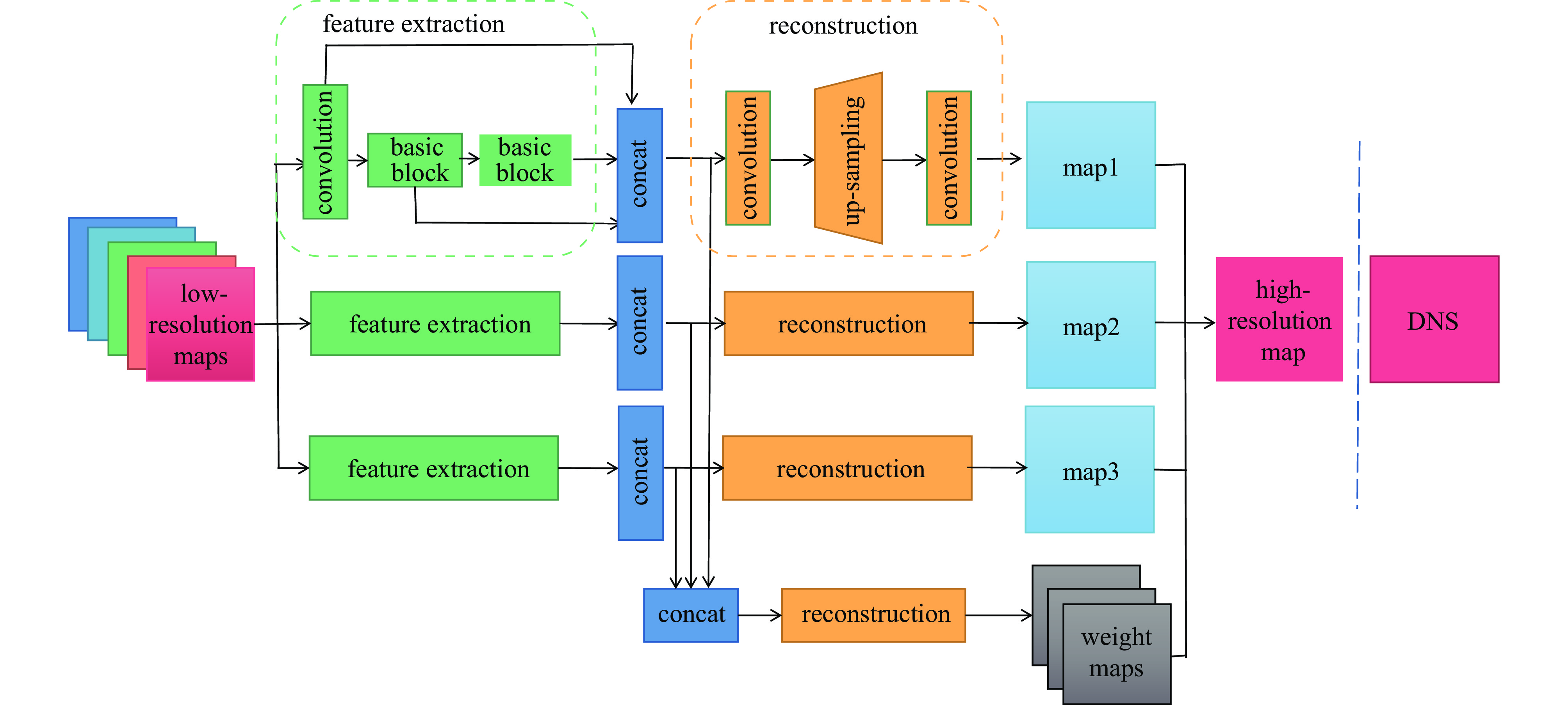
Ld=12μm . Firstly, the velocity field is reconstructed by using the data of the two channels in the x, y directions as the input of the model. The training error and test set error of the ordinary CNN model and the multiple CNN model are shown in Fig.3. Figure 3. Error maps of two convolutional neural network models
In Fig.3, CNN represents the ordinary CNN, MTPC represents the multi-time-path CNN, training loss refers to the training set error, and testing loss refers to the test set error. Compared with the ordinary CNN, the error of the multi-time-path CNN is smaller, reduced by nearly 10 times. It can be said that the multi-time-path CNN has better reconstruction performance than the ordinary CNN.
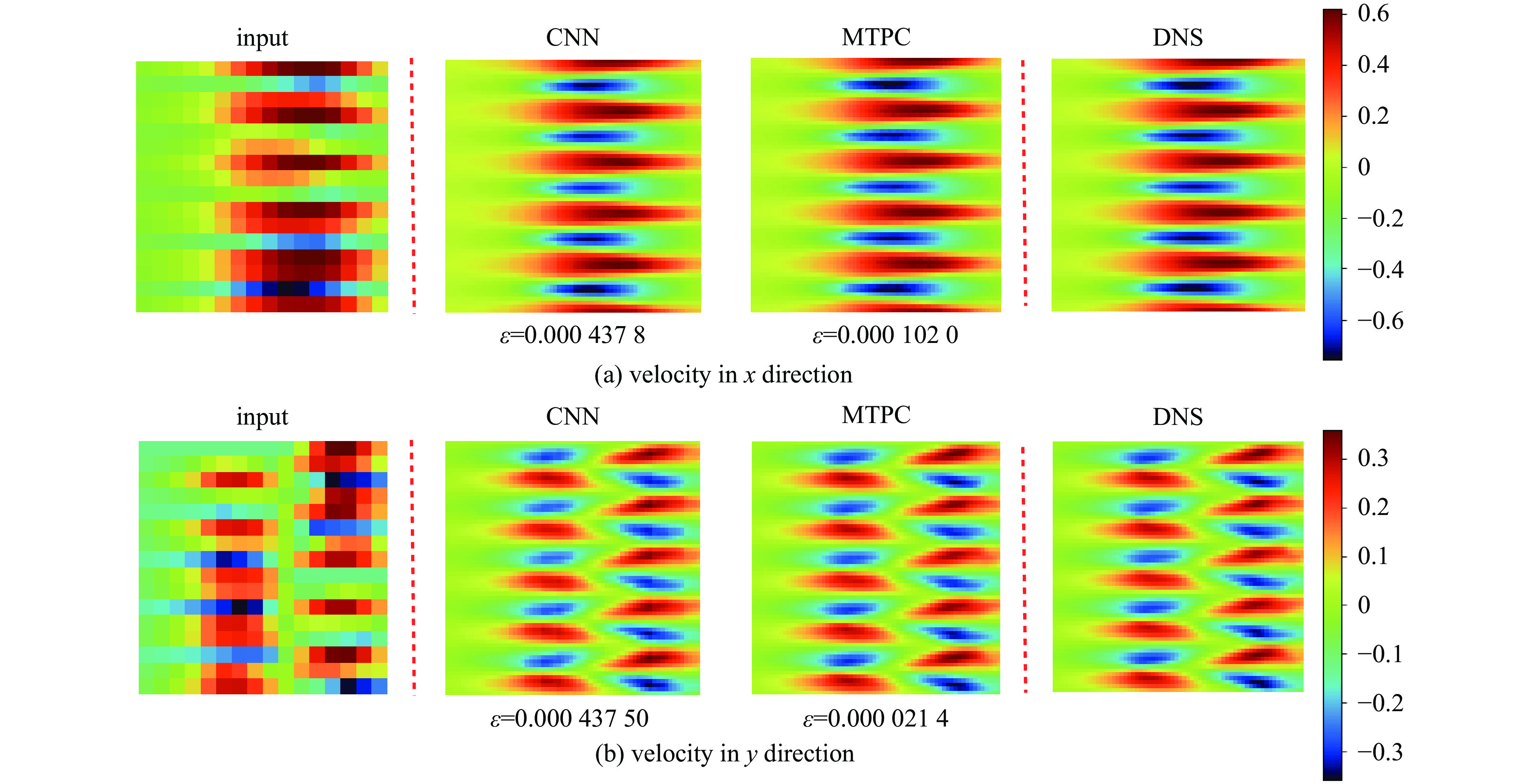
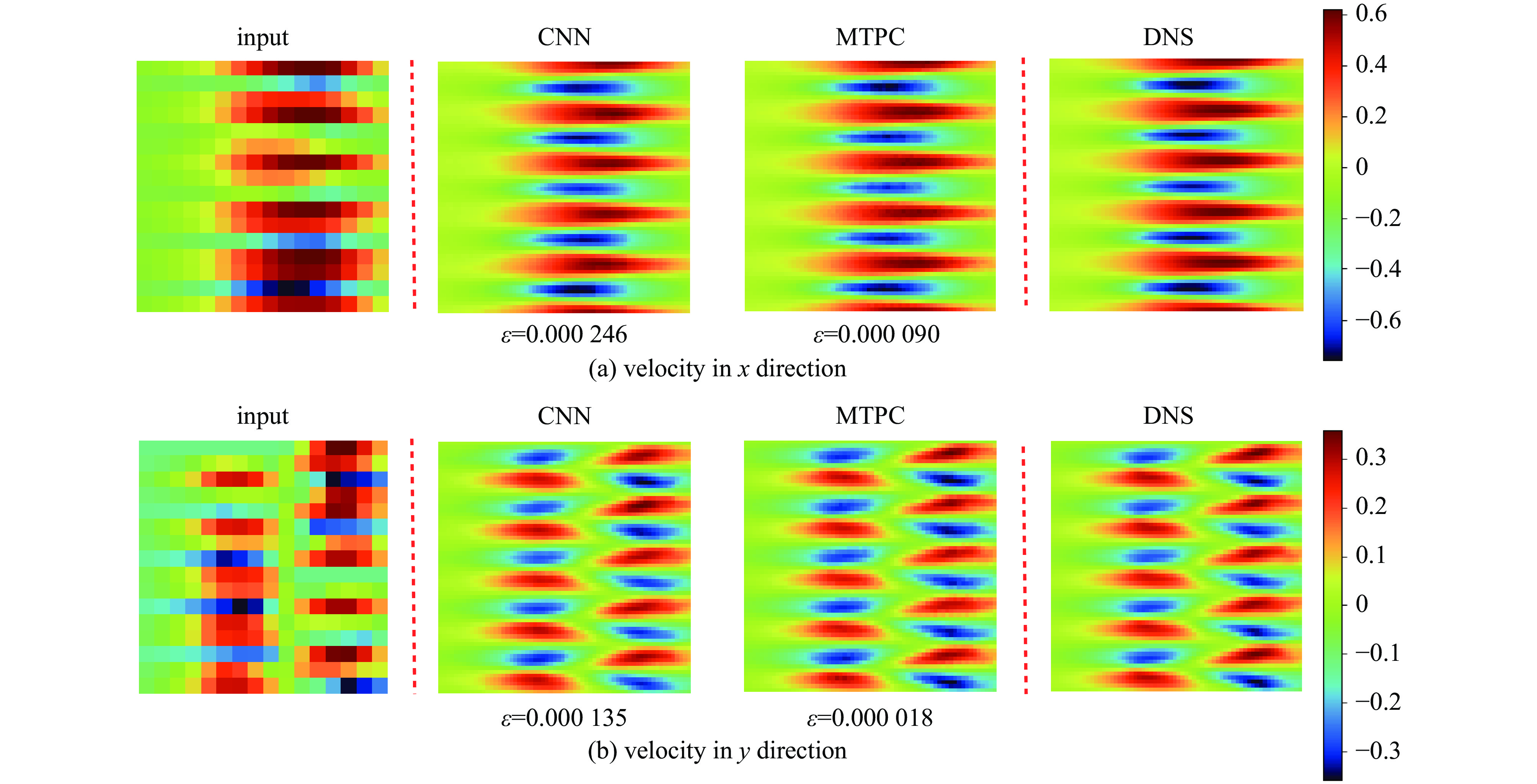
To more clearly show the superiority of the multi-time-path CNN, we compare the reconstructed results of the two models. All the data shown in Fig.4 and Fig.5 come from the same flow field,which are the flow field velocity data of the same position at the same time.
 Figure 4. Comparison of reconstructed results with average pooling (r=4)
 Figure 5. Comparison of reconstructed results with maximum pooling (r=4)
Fig.4 is the comparison of the reconstruction results when the input is the flow field velocity data in x and y directions after average pooling. Fig.5 is the comparison of the reconstruction results when the input is the flow field velocity data in two directions after maximum pooling. The reconstruction magnification r of the two figures is 4, and the
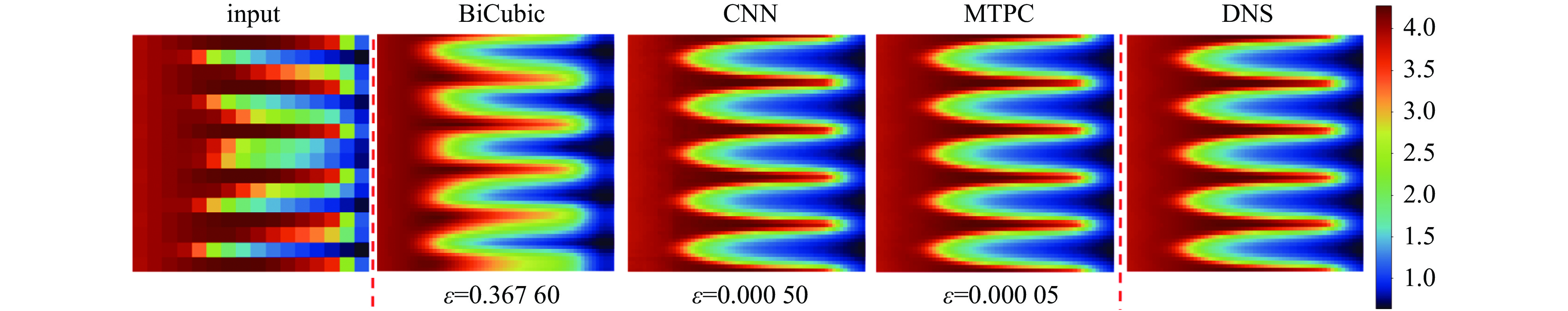
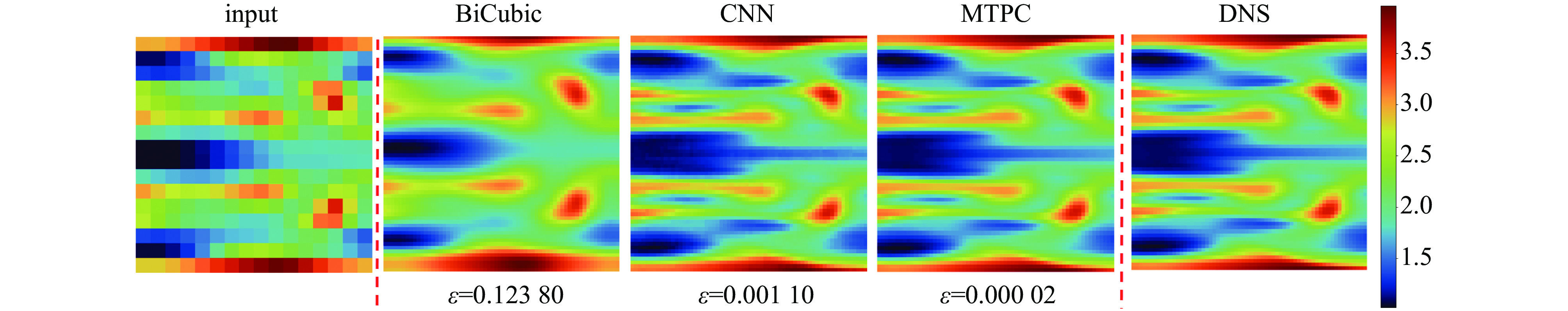
ε in the figure is the MSE. It can be clearly seen that the MSE of the multi-time-path CNN is much smaller than that of the ordinary CNN for both the average pooling case and the maximum pooling case. To show that the performance of the multi-time-path CNN is better than that of the ordinary CNN, we also compare the reconstruction results of models with magnification r= 8. The results show that even when the magnification r is 8, the error of the multi-time-path CNN is still much smaller than that of the ordinary CNN. Compared with the case of magnification r being 4, the error increases when the magnification r is 8, which is also in line with expectations: as the magnification increases, the amount of input data decreases, and the error of the model should also increase. Comparing the results of average pooling and maximum pooling, average pooling will lead to smooth prediction results but reduce accuracy, while maximum pooling can retain more details and help to improve prediction accuracy, but the results are not as smooth as average pooling.Furthermore, the density of the flow field is also used for training the model as a separate input. To demonstrate the universality of the model, we analyze the flow field density data of four cases (r=4). The first case is the density data of the weak nonlinear stage with ablation (disturbance wavelength=12 μm), as shown in Fig.6.
 Figure 6. Comparison of the high-resolution reconstructed density data (weak nonlinear stage with ablation, disturbance wavelength=12 μm)
BiCubic in Fig.6 denotes the results of the BiCubic interpolation reconstruction method, and the BiCubic interpolation method is widely used in image processing. The prediction results of the BiCubic interpolation method exhibit excessive smoothness, resulting in the loss of numerous detailed characteristics within the flow field. It can be clearly seen from Fig.6 that the performance of both ordinary CNN and multi-time-path CNN in high-resolution reconstruction of flow field data is far superior to that of BiCubic interpolation method. The multi-time-path CNN consistently demonstrates superior performance compared to the ordinary CNN, effectively recovering more flow field details with a lower error.
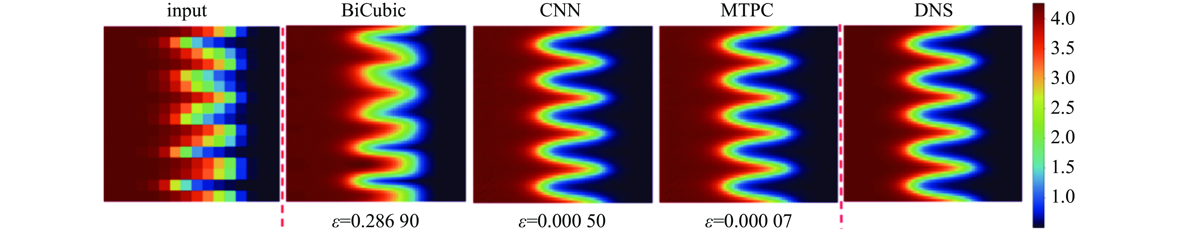
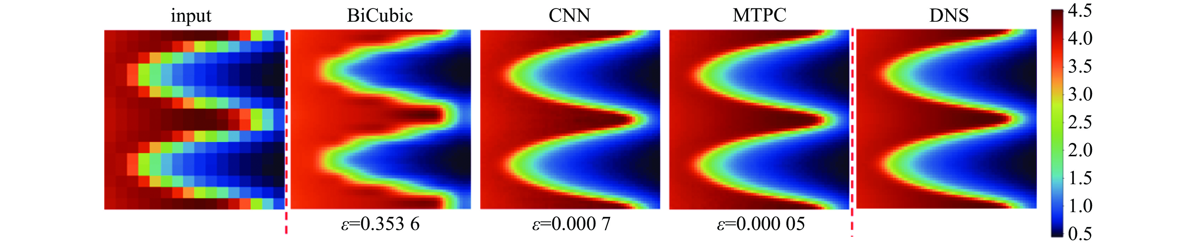
Fig.7 is the classical linear flow field density data (disturbance wavelength=12 μm), and Fig.8 is the density data of the nonlinear stage with ablation (disturbance wavelength=12 μm). In addition, we also discuss the flow field with the disturbance wavelength of 30 μm, as shown in Fig.9.
 Figure 7. Comparison of the high-resolution reconstructed density data (classical linear stage, disturbance wavelength=12 μm)
 Figure 8. Comparison of the high-resolution reconstructed density data (nonlinear stage with ablation, disturbance wavelength=12 μm)
 Figure 9. Comparison of the high-resolution reconstructed density data (weak nonlinear stage with ablation, disturbance wavelength=30 μm)
In these cases, the prediction error of the multi-time-path CNN is generally at the order of 10−5, while the error of the ordinary CNN is at the order of 10−4. Both of these errors are significantly lower than that of the the BiCubic interpolation method. It is shown by these cases that the multi-time-path CNN still exhibits excellent performance in the face of different flow parameters, different stages and different flow field data.
For the velocity component input case and the density component input case, the error of reconstructing the flow field based on multi-time-path CNN is low enough, and the performance is sufficiently good. This also fully demonstrates the feasibility of combining machine learning with fluid mechanics. The methods used in this paper can also be applied to other flow field data. Given a sufficient amount of flow field data, a corresponding high-resolution reconstruction model can be trained.
3. Conclusion
We have built an ordinary CNN and a multi-time-path CNN to achieve high-resolution reconstruction of the low-resolution ablation Rayleigh-Taylor instability flow field. Compared with the ordinary CNN, the multi-time-path CNN shows better performance and smaller error. In terms of the acquisition of input data, we first pooled the existing high-precision DNS data of our research group to obtain low-resolution flow field data, and then we performed dislocation splicing on the data to obtain training sample data. The influence of input data obtained by two pooling methods on model training is compared. The prediction results of the average pooling model are smoother, and the accuracy of the maximum pooling model is slightly higher. Different cases are discussed in this paper, and it is found that the multi-time-path CNN model still maintains excellent performance in different flow fields. Once the CNN model is trained, the high-resolution reconstruction task can be completed in just a few seconds. The introduction of these two models has enriched the application of CNN in fluid instability. With the development of computer technology, the training speed of CNN model will be faster and faster. We can construct more complex models to make the reconstruction accuracy higher and higher.
-
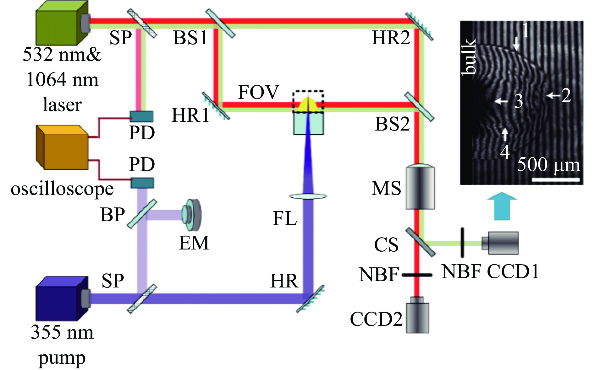
图 1 双波长干涉实验光路
Figure 1. Schematic of interference imaging system with dual-wavelength probes
BS, beam splitter; HR, reflector; SP, beam sampler; CS, color separator; PD, photon detector; EM, energy meter; NBF, narrow band filter; MS, microscope; FL, focus lens
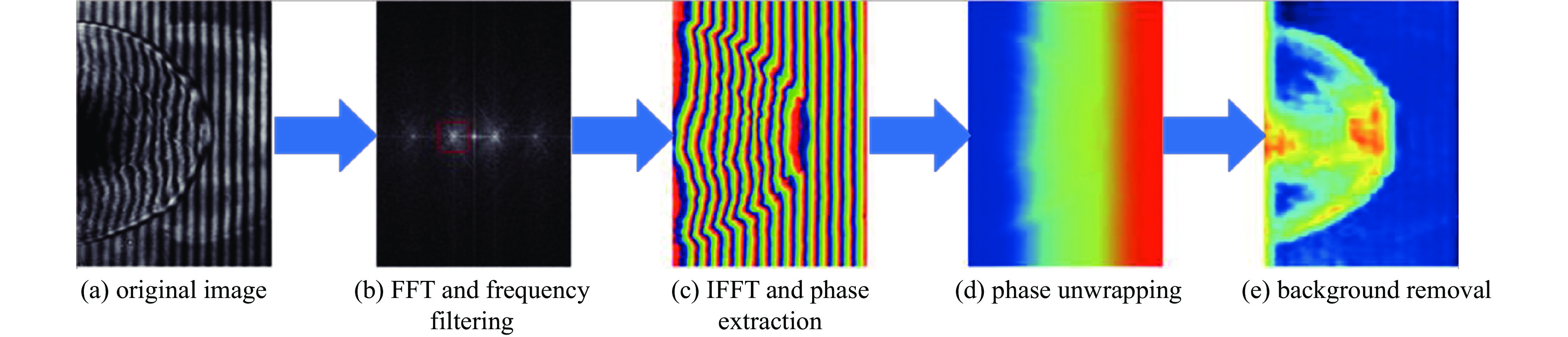
图 2 干涉图像获取流场信息提取流程
Figure 2. Extraction processing of phase shift information of interference image
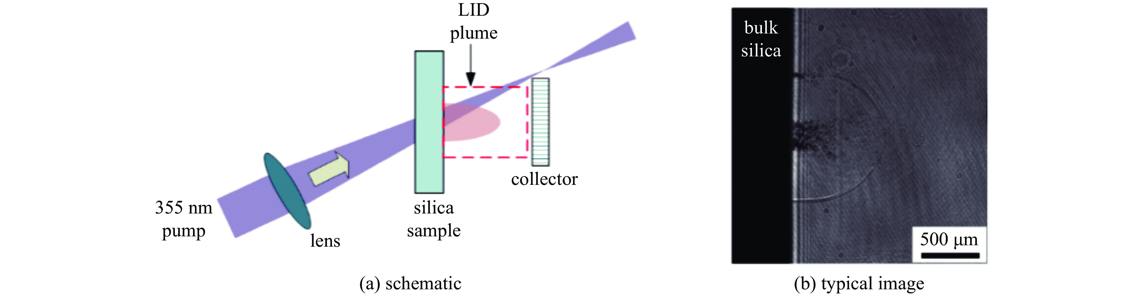
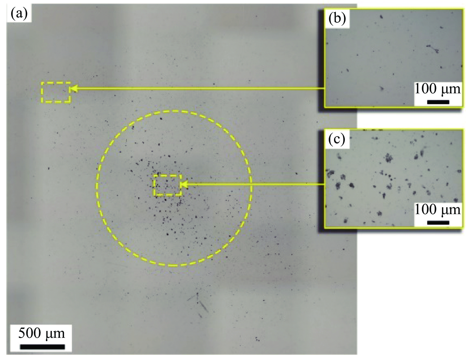
图 3 喷溅颗粒收集设置示意图及喷溅颗粒流的典型图像
Figure 3. Schematic of ejected particle collecting setup and typical image of the particle jets
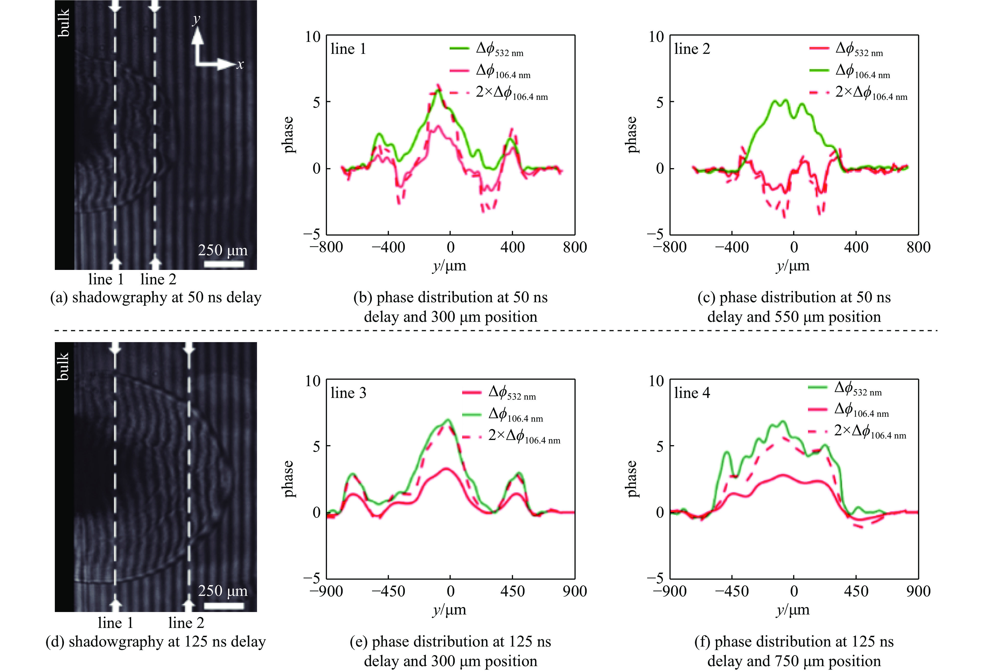
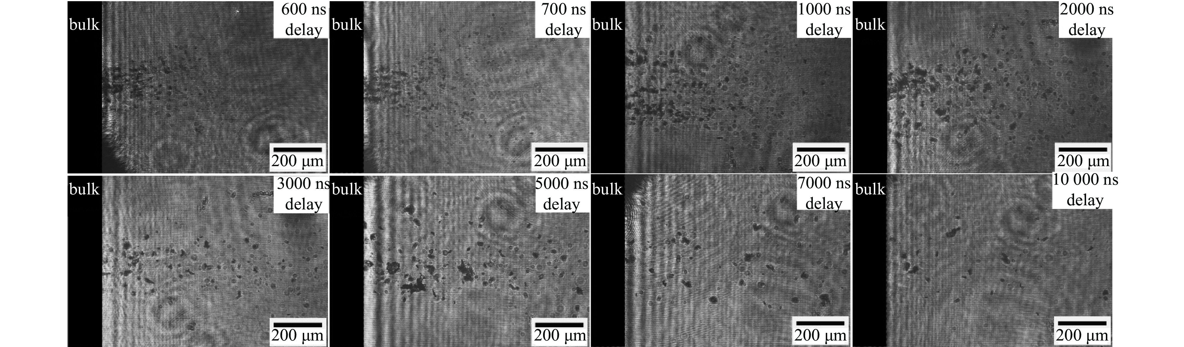
图 5 后表面不同位置处的双波长探针相位偏移横向分布
Figure 5. Lateral distribution of phase shift of dual-wavelength probe at different position from rear surface inside damage plume
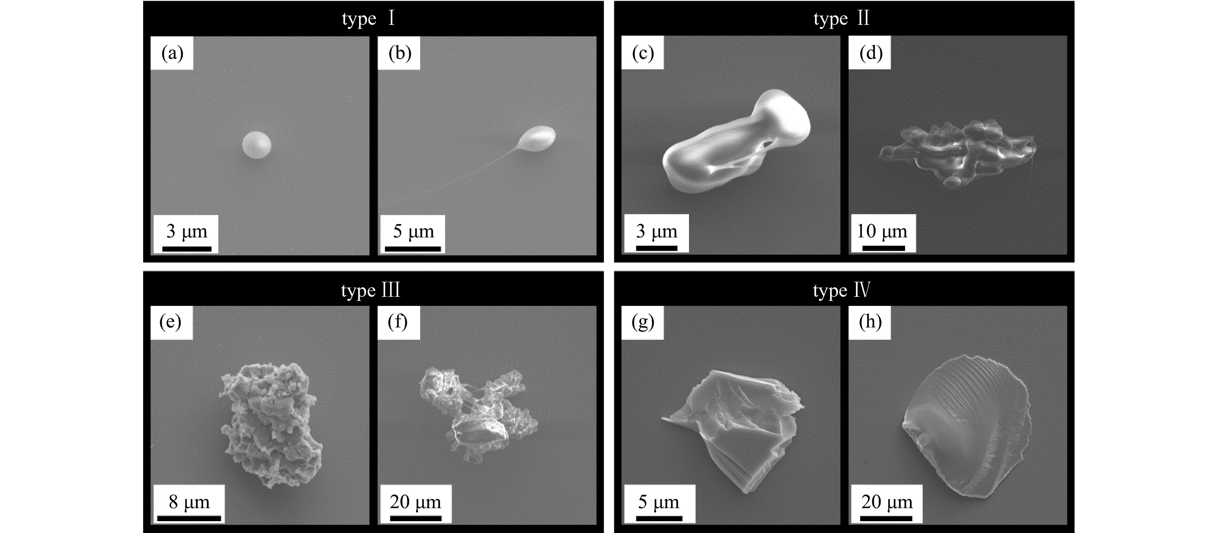
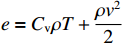
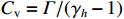
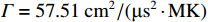
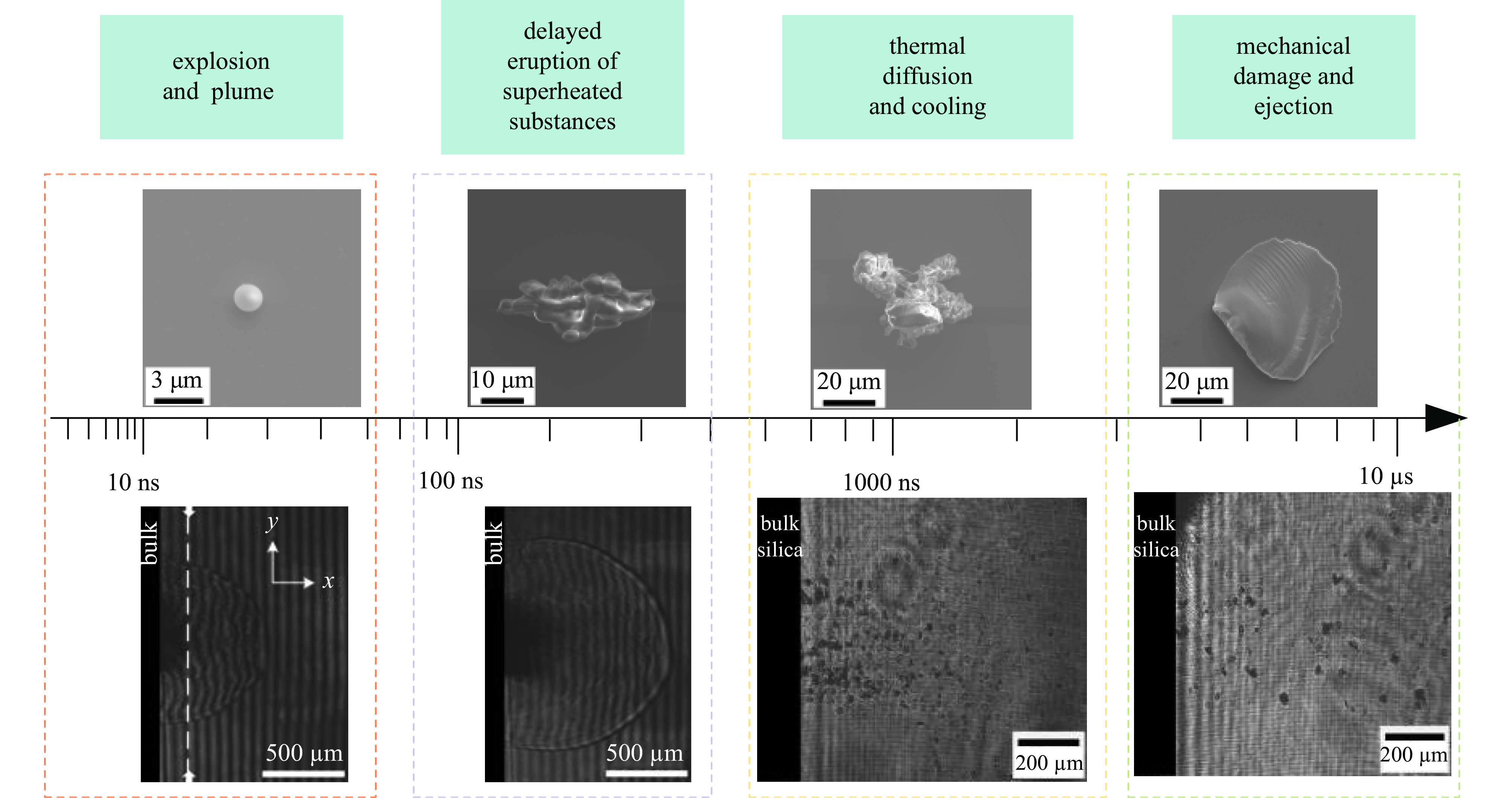
图 7 熔石英后表面紫外损伤的颗粒喷溅物的SEM图像
Figure 7. SEM images of particle ejection generated by UV laser induced rear surface damage of fused silica
-
[1] Spaeth M L, Wegner P J, Suratwala T I, et al. Optics recycle loop strategy for NIF operations above UV laser-induced damage threshold[J]. Fusion Science and Technology, 2016, 69(1): 265-294. doi: 10.13182/FST15-119 [2] Chambonneau M, Lamaignère L. Multi-wavelength growth of nanosecond laser-induced surface damage on fused silica gratings[J]. Scientific Reports, 2018, 8(1): 891. doi: 10.1038/s41598-017-18957-9 [3] Negres R A, Cross D A, Liao Z M, et al. Growth model for laser-induced damage on the exit surface of fused silica under UV, ns laser irradiation[J]. Optics Express, 2014, 22(4): 3824-3844. doi: 10.1364/OE.22.003824 [4] Negres R A, Norton M A, Cross D A, et al. Growth behavior of laser-induced damage on fused silica optics under UV, ns laser irradiation[J]. Optics Express, 2010, 18(19): 19966-19976. doi: 10.1364/OE.18.019966 [5] Laurence T A, Negres R A, Ly S, et al. Role of defects in laser-induced modifications of silica coatings and fused silica using picosecond pulses at 1053 nm: II. Scaling laws and the density of precursors[J]. Optics Express, 2017, 25(13): 15381-15401. doi: 10.1364/OE.25.015381 [6] Negres R A, Raman R N, Bude J D, et al. Dynamics of transient absorption in bulk DKDP crystals following laser energy deposition[J]. Optics Express, 2012, 20(18): 20447-20458. doi: 10.1364/OE.20.020447 [7] Raman R N, Negres R A, Demos S G. Kinetics of ejected particles during breakdown in fused silica by nanosecond laser pulses[J]. Applied Physics Letters, 2011, 98: 051901. doi: 10.1063/1.3549193 [8] Demos S G, Negres R A, Raman R N, et al. Material response during nanosecond laser induced breakdown inside of the exit surface of fused silica[J]. Laser & Photonics Reviews, 2013, 7(3): 444-452. [9] Demos S G, Negres R A, Raman R N, et al. Relaxation dynamics of nanosecond laser superheated material in dielectrics[J]. Optica, 2015, 2(8): 765-772. doi: 10.1364/OPTICA.2.000765 [10] Kanitz A, Kalus M R, Gurevich E L, et al. Review on experimental and theoretical investigations of the early stage, femtoseconds to microseconds processes during laser ablation in liquid-phase for the synthesis of colloidal nanoparticles[J]. Plasma Sources Science and Technology, 2019, 28: 103001. doi: 10.1088/1361-6595/ab3dbe [11] 赵元安, 邵建达, 刘晓凤, 等. 光学元件的激光损伤问题[J]. 强激光与粒子束, 2022, 34:011004 doi: 10.11884/HPLPB202234.210331Zhao Yuan’an, Shao Jianda, Liu Xiaofeng, et al. Tracking and understanding laser damage events in optics[J]. High Power Laser and Particle Beams, 2022, 34: 011004 doi: 10.11884/HPLPB202234.210331 [12] 杨李茗, 黄进, 刘红婕, 等. 熔石英元件紫外脉冲激光辐照损伤特性研究进展综述[J]. 光学学报, 2022, 42:1714004 doi: 10.3788/AOS202242.1714004Yang Liming, Huang Jin, Liu Hongjie, et al. Review of research progress on damage characteristics of fused silica optics under ultraviolet pulsed laser irradiation[J]. Acta Optica Sinica, 2022, 42: 1714004 doi: 10.3788/AOS202242.1714004 [13] Huang Jin, Liu Hongjie, Wang Fengrui, et al. Influence of bulk defects on bulk damage performance of fused silica optics at 355 nm nanosecond pulse laser[J]. Optics Express, 2017, 25(26): 33416-33428. doi: 10.1364/OE.25.033416 [14] 郑万国, 祖小涛, 袁晓东, 等. 高功率激光装置的负载能力及其相关物理问题[M]. 北京: 科学出版社, 2014Zheng Wanguo, Zu Xiaotao, Yuan Xiaodong, et al. Damage resistance and physical problems of high power laser facilities[M]. Beijing: Science Press, 2014 [15] Demos S G, Negres R A, Rubenchik A M. Dynamics of the plume containing nanometric-sized particles ejected into the atmospheric air following laser-induced breakdown on the exit surface of a CaF2 optical window[J]. Applied Physics Letters, 2014, 104: 031603. doi: 10.1063/1.4862815 [16] Nguyen V H, Kalal M, Suk H, et al. Interferometric analysis of sub-nanosecond laser-induced optical breakdown dynamics in the bulk of fused-silica glass[J]. Optics Express, 2018, 26(12): 14999-15008. doi: 10.1364/OE.26.014999 [17] Demos S G, Raman R N, Negres R A. Time-resolved imaging of processes associated with exit-surface damage growth in fused silica following exposure to nanosecond laser pulses[J]. Optics Express, 2013, 21(4): 4875-4888. doi: 10.1364/OE.21.004875 [18] Peng Ge, Zhang Peng, Dong Zhe, et al. Spatial sputtering of fused silica after a laser-induced exploding caused by a 355 nm nd: YAG laser[J]. Frontiers in Physics, 2022, 10: 980249. doi: 10.3389/fphy.2022.980249 [19] Bude J, Guss G, Matthews M, et al. The effect of lattice temperature on surface damage in fused silica optics[C]//Proceedings of SPIE 6270, Laser-induced Damage in Optical Materials. 2007. [20] Zhu Chengyu, Liang Lingxi, Yuan Hang, et al. Investigation of stress wave and damage morphology growth generated by laser-induced damage on rear surface of fused silica[J]. Optics Express, 2020, 28(3): 3942-3951. doi: 10.1364/OE.384036 -


 DownLoad:


 下载:
下载:

 点击查看大图
计量
- 文章访问数: 714
- HTML全文浏览量: 287
- PDF下载量: 106
- 被引次数: 0
